Dashboard Apps
The ilumr dashboard apps allow you to monitor and calibrate the system, and run simple NMR and MRI experiments with just a few button clicks.
To find the dashboard apps, click the ilumr symbol in the Jupyter Lab interface’s left panel.
App Tools and Features
Most of the apps share common tools and features, and it is useful to familiarise yourself with these common features before you begin exploring each app.
Running Apps
Most dashboards have a control bar with the following features:
Run - Click the green “Run” button to run a dashboard. This button will grey out while the dashboard is running. While a dashboard is running, all other dashboards will be disabled.
Abort - Click the red “Abort” button to stop a dashboard that is running.
Progress Bar - This bar shows the estimated progress in green.
Status Bar - This bar will display the dashboard’s current status and error messages.
Dashboard Features
Common status messages are:
Running - The dashboard is currently running, even if there is not visible progression on the progress bar.
Finished - The dashboard has completed its process.
Busy - A dashboard is running elsewhere, therefore, the system is busy and the dashboard you are trying to use can not run. You will need to check the other dashboards you have open and find the dashboard with a “Running” status. Once you have located the dashboard that is running, press “Abort” on this dashboard. You may now return to the previous dashboard you were trying to use and press “Run”.
Navigating Plots
The plots generated within dashboards are interactive bokeh plots and have the following features which can be toggled by clicking their icons.
Plot Features
Left click and drag to pan
Select area to zoom
Zoom with mouse wheel, position within plot to zoom both axes or over an individual axis (orange points) to zoom in on a single axis
Reset the plot
Save a PNG (follows browser settings for downloads)
Toggle crosshairs
Saving Data
Data from the dashboard apps can be saved using the save options located beneath the control bar.
Data Saving Features
Saving Directory - will save the data to “user/data/<Workspace>/<File Name>”. Subdirectories can also be specified using a “/”, e.g. “lab_1/ilumr_workspace” to save to “user/data/lab_1/ilumr_workspace/<File Name>”.
File Name - will save with this file name within the chosen workspace directory.
Save - save the data (data will not be autosaved).
When you save data from the dasboard apps, two files will be saved. The first file is a “.npy” file which contains the k-space data from the experiment and the second file is a “.yaml” file which contains the pulse sequence parameters that were used in the experiment.
Autosaved Parameters
The dashboard apps used for configuring and setting up the instrument will automatically update system parameters when executed. These system parameter sets can be found in files in the “globals” directory. These files are not intended to be changed manually under normal circumstances.
System and Calibration Apps
When you first set up your ilumr, it is important to run through the system and calibration apps in the order they are presented in this user guide. This will ensure that your system has been properly prepared before you begin your magnetic resonance experiments.
Attention
To prepare the system for calibration, please place the supplied shim sample into ilumr. Ensure the entire sample is contained within the homogenous region of the magnet.
Admin
This dashboard is not part of the setup process but is important to take note of as it controls two key functions: Shutting Down the System and Installing Updates
Admin Dashboard
Shutting Down ilumr
When you want to shut down the system, simply check the “Enable Shutdown” checkbox (1) and click the red “Shutdown” button (2).
Attention
To avoid data loss, please always use the admin dashbaord when you need to shutdown ilumr. Please do NOT use the power button on the front of the system for shutdown purposes.
Installing Updates
When you want to install updates:
Plug ilumr into a router with internet access using an ethernet cable.
Connect to ilumr via wifi or its IP address assigned by the router.
Open the “Admin” Dashboard App.
Click the “Enable Shutdown/Update” checkbox (1).
Press the blue “Update” button (3) at the bottom of the dashboard.
A “Server Connection Error” will show as the JupyterLab server is stopped during the update process.
Leave ilumr powered until JupyterLab restarts. This will take about 10 minutes, depending on the internet speed. You may need to reload the page to check if it is done.
Temperature
The first step in the ilumr setup process is to check the Temperature dashboard. The magnet in ilumr is temperature controlled to keep the system frequency stable and uses a PT100 sensor to measure its temperature. The sensor results are displayed on the dashboard.
Temperature Dashboard
Note
The set control point is 30°C, please ensure that the system has reached and held 30°C for at least 30 minutes before continuing with the setup process.
Noise Check
Once the system temperature is stable, you can perform a Noise Check. This dashboard allows you to assess whether the operating environment is suitable for ilumr with no large sources of electrical interference. When you run this dashbaord the system will measure and display the environmental noise level.
Click Run for a single measurement or Run Loop for continuous measurements.
Interference will show up as large spikes extending higher then the baseline noise level. The RMS of the noise signal is displayed in the top left, and should be less than 0.5 µV when using a dwell time of 1 µs.
If the noise signal is higher than 0.5 µV, try moving noise sources (like powerboards/multiboxes and other electronincs) away from ilumr.
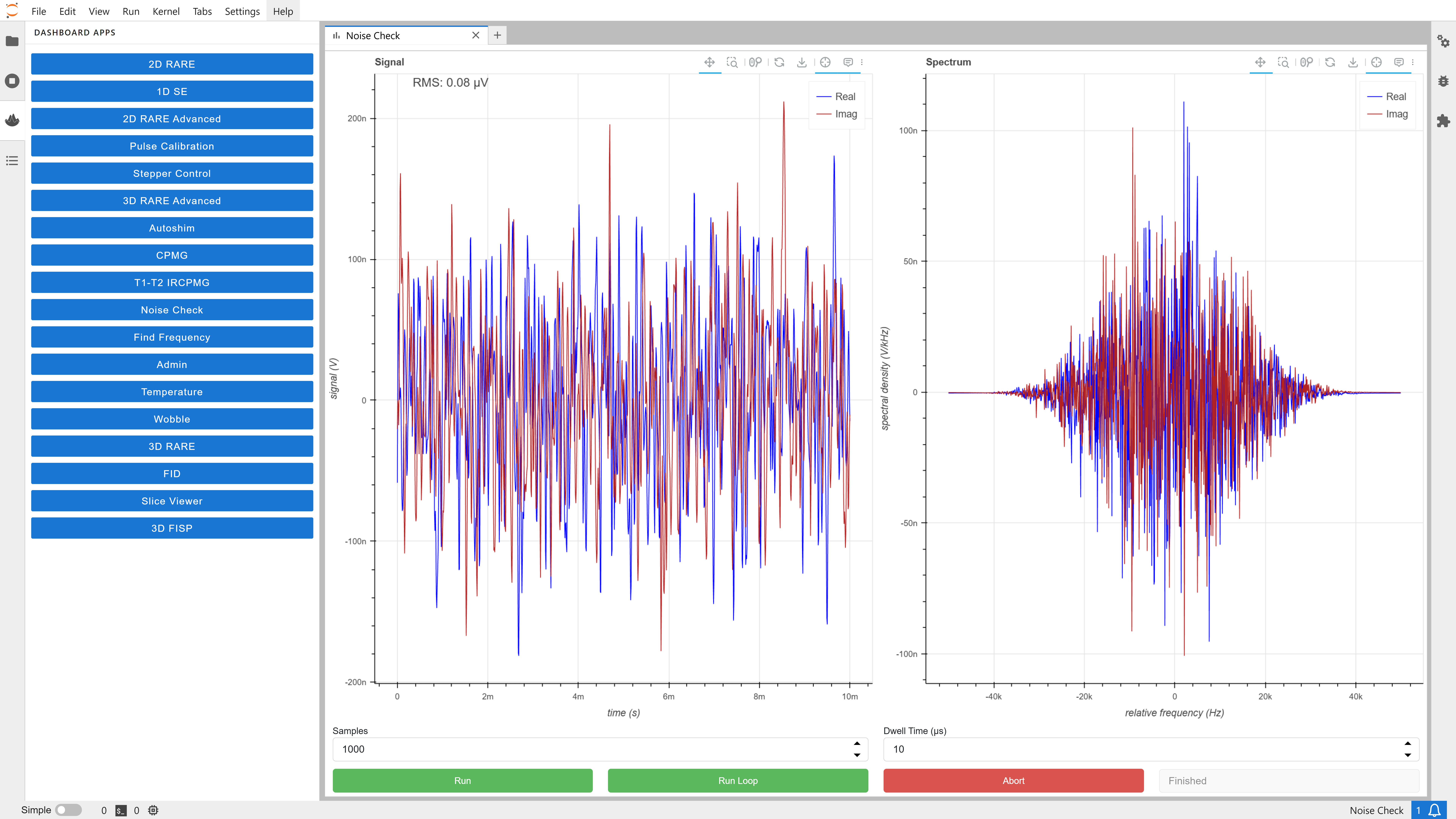
Noise Check Dashboard
Note
Note that the data shown here is raw data from the hardware decimator, which does not have a flat frequency response, so the noise spectrum (right-hand plot) will normally have a bell-curve-like shape as shown below.
Find Frequency
The next dashboard to run is Find Frequency which uses an free induction decay (FID) pulse sequence with several dwell time increments in order to determine the NMR frequency of the magnet.
Begin by aligning the provided shim sample with the window in the depth gaude then inser the sample into the system. Press Run to perform the experiment and determine the NMR frequency. The new frequency value is automatically saved and can be found in the following location:
globals/frequency.yaml
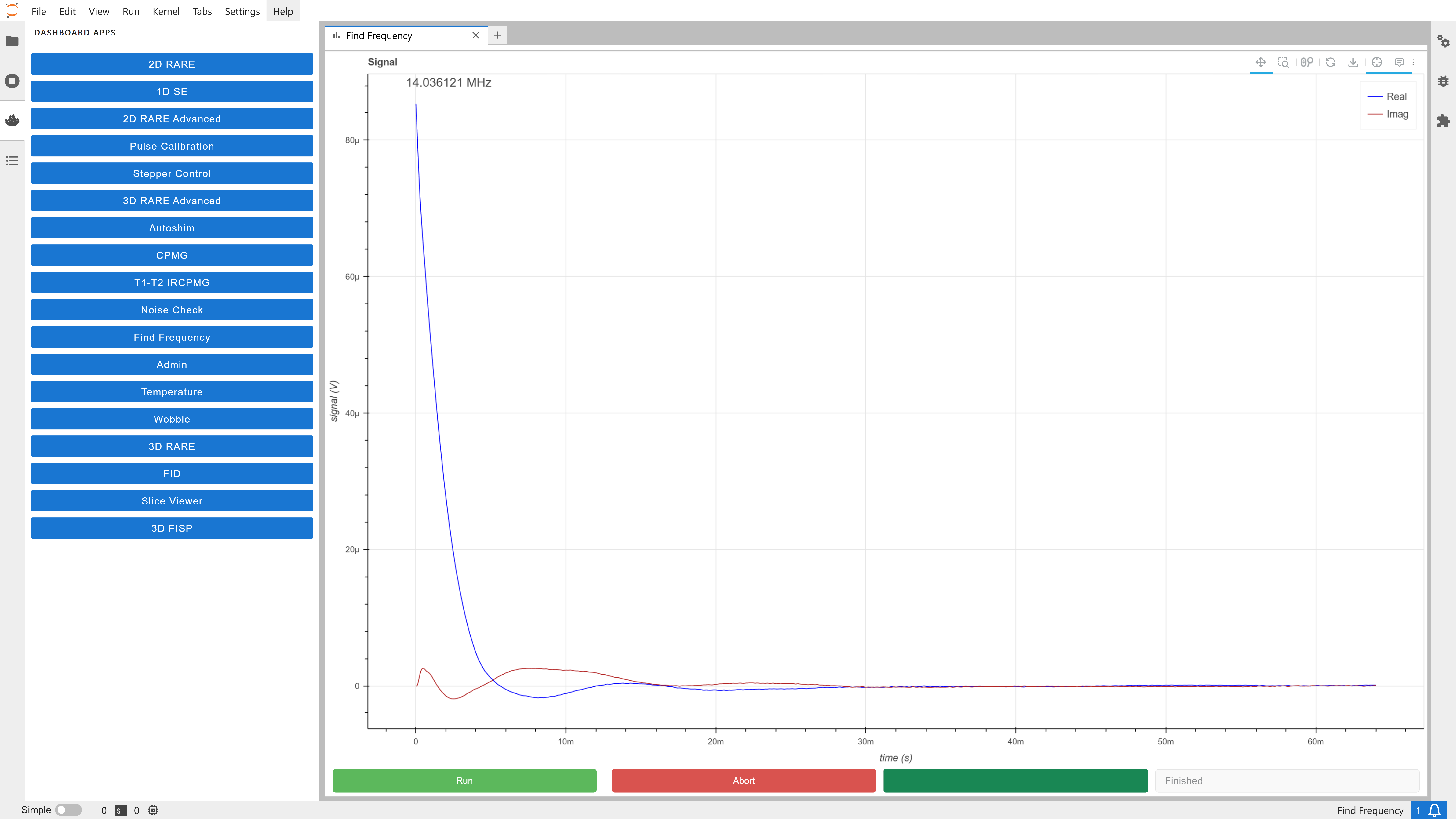
Frequency Dashboard
Wobble
The RF probes supplied with ilumr have been tuned to the magnet’s resonant frequency. However, due to differences in operating environments, this frequency may shift slightly. It is important to have the probe tuned to the current magnet frequency. Before running NMR experiments, use the Wobble dashboard to check and adjust the probe tuning if required.
In the graph below, the dotted line indicates the magnet frequency, taken from the frequency found in the previous dashboard. This is an example of a well tuned probe, small offsets from the NMR frequency are not a problem and may also be caused by a change in sample. Try removing the shim sample while running the wobble in looped mode to see the effect.
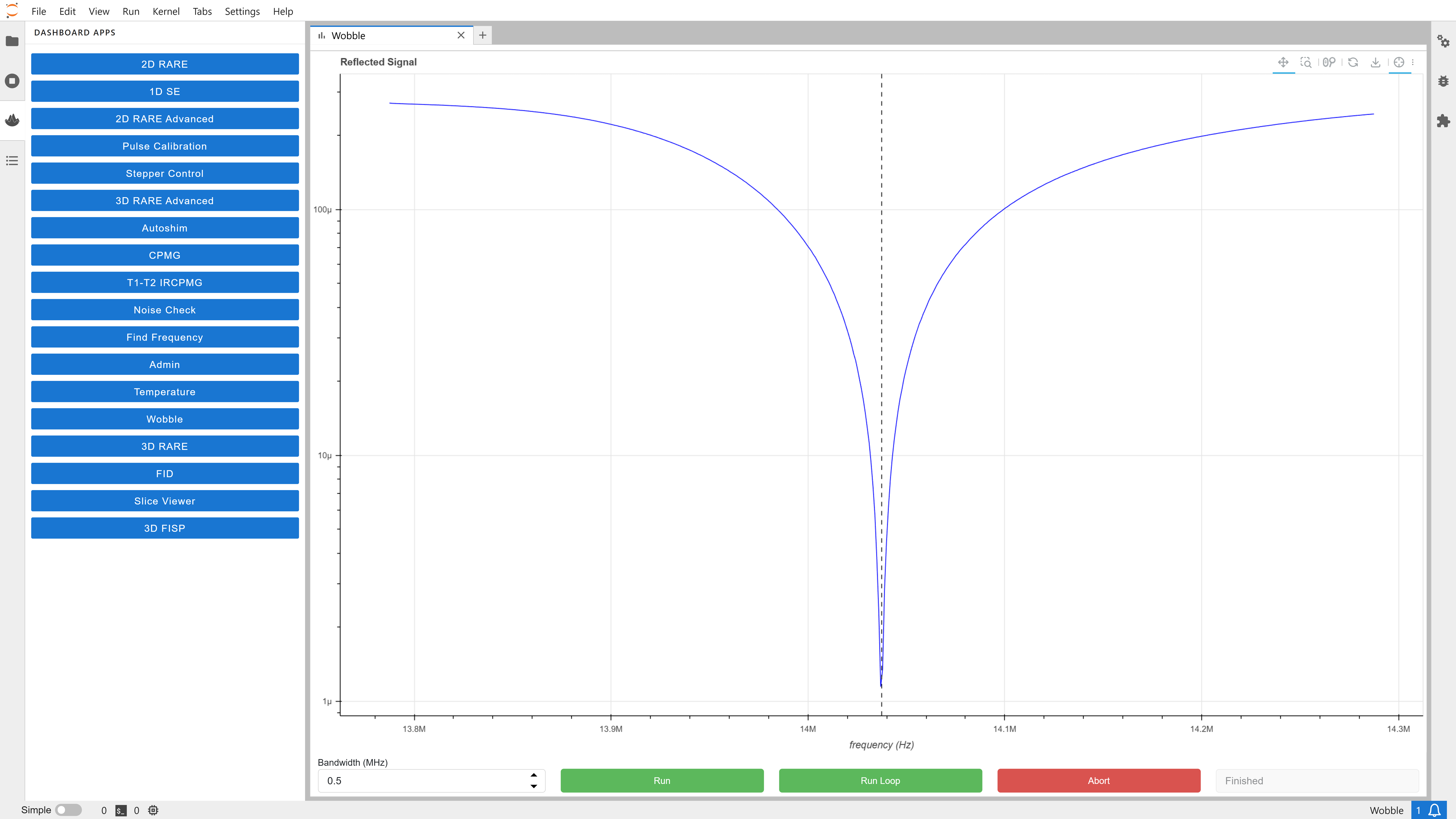
Wobble Dashboard
A well tuned probe should meet the following requirements:
Tune: NMR frequency +/- 0.02MHz
Match: less then 20 µV (20e-6) at NMR frequency
If the probe tunings falls outside of these requirements, please follow the next steps:
Click “Run Loop” on the Wobble dashboard.
Remove the top disk by rotating anti-clockwise
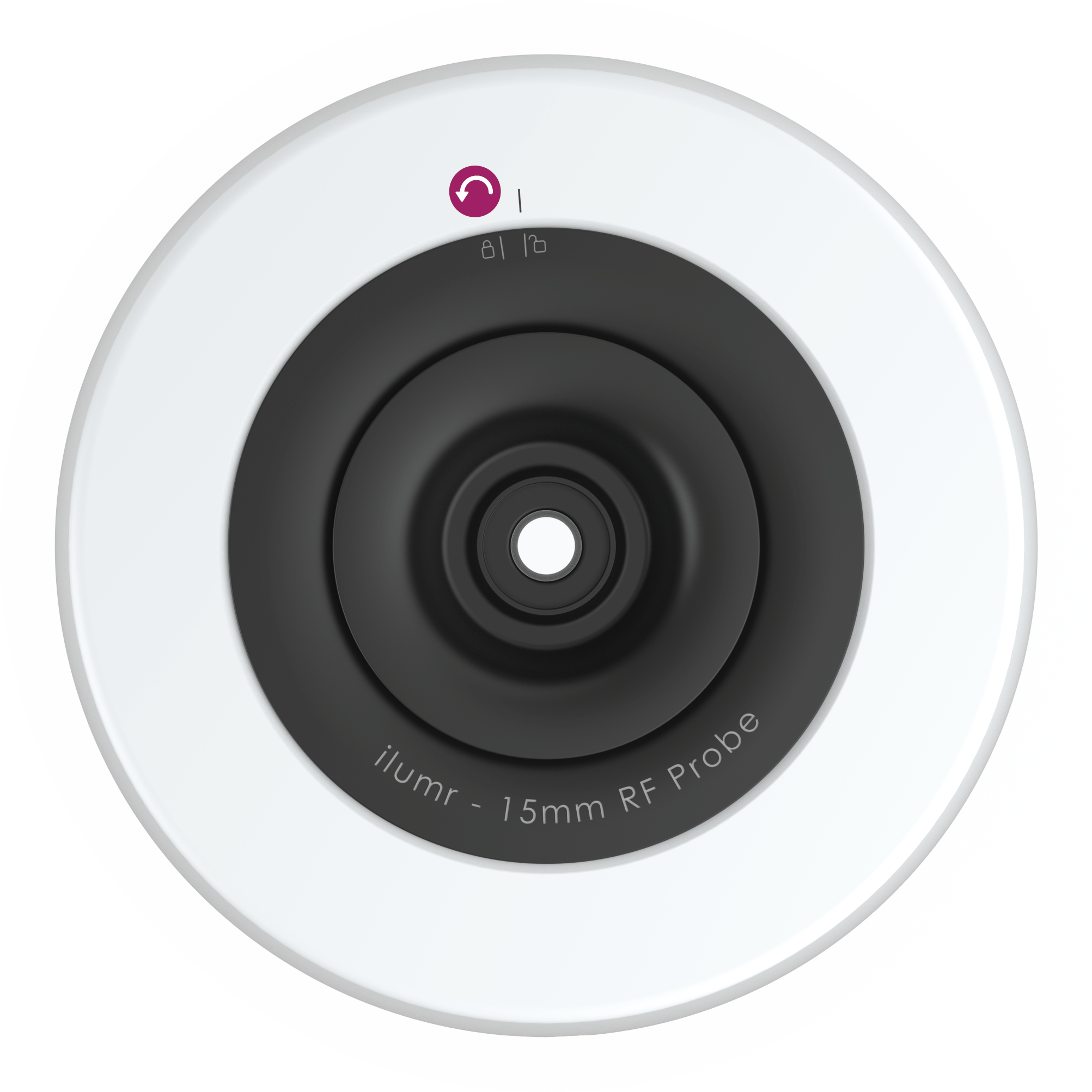
ilumr Top Disk
Identify the tune (1) and match (2) capacitors using the provided image. The bottom tune/match capacitor is for coarse adjustment and the top for fine adjustment.
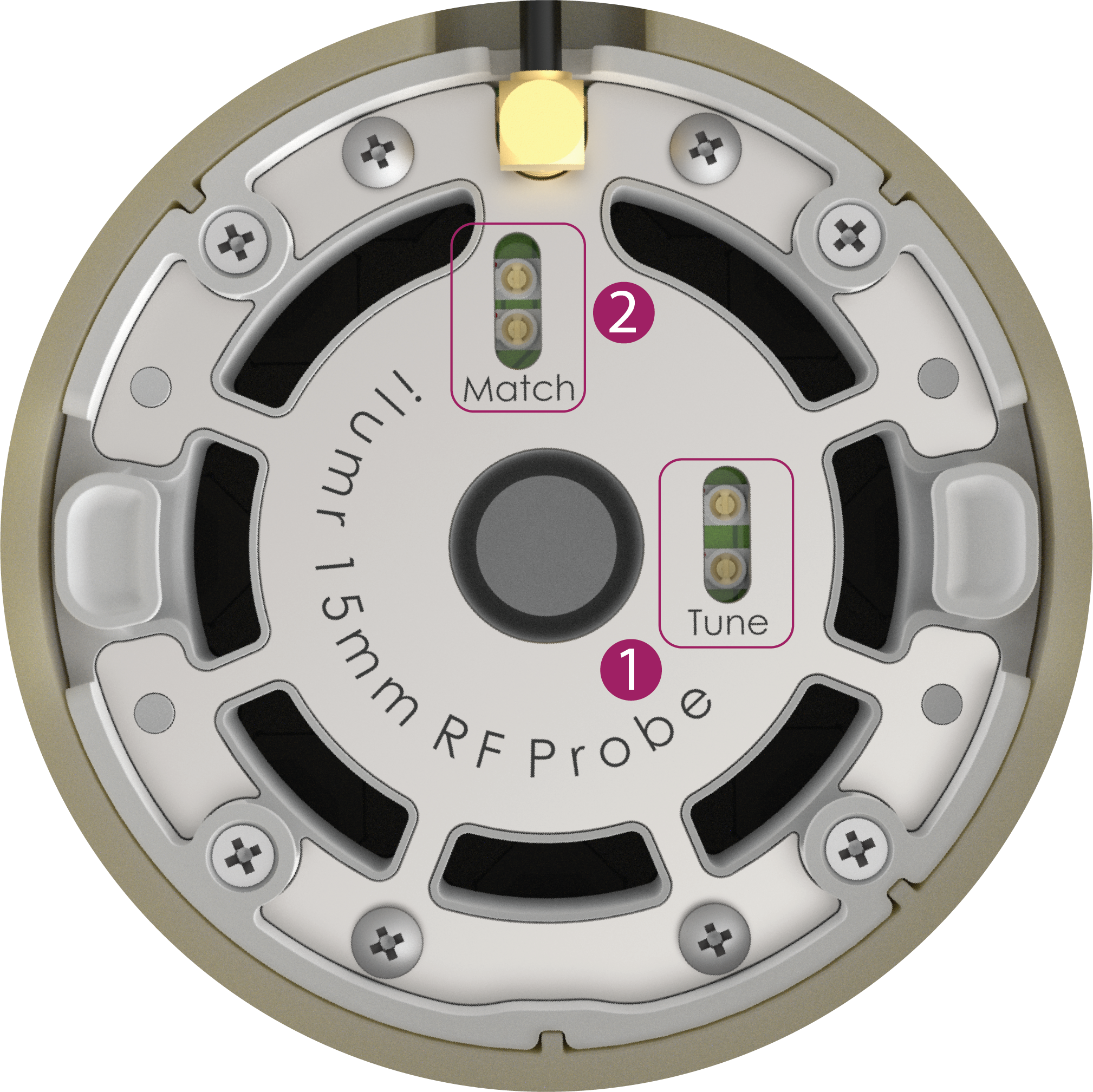
ilumr Tune and Match Capacitors
Identify the alignment arrows and notches on the capacitors. Each capacitor has a tiny arrow on the turning part and a notch on the rim. One end of the adjustment range is reached when the arrow is aligned with the notch, and the other end is reached when the arrow is pointing in the opposite direction.
Use the supplied trimmer too to adjust the fine capacitors to 90° from the notch (the halfway point of its range).
Adjust the coarse capacitors to get the tune/match roughly correct.
Then use the fine capacitors to refine the tune/match.
Note
Note that the presence of the trimmer tool will shift the value so remove after each small adjustment to check.
Pulse Calibration
Once the tuning/matching of the probe has been confirmed, the pulse power of 90 and 180 degree RF pulses can be calibrated using the Pulse Calibration dashboard.
The default settings should be adequate when using the 11 mm RF probe (provided as default with ilumr), but the 15 mm RF probe will require a longer Pulse Width (recommended 60 us) and a greater Number of Steps (recommended 100) to achieve a 180 degree tipping angle.
Click Run to begin the pulse calibration algorithm.
Once pulse calibration is complete, vertical dotted lines will show the amplitudes of the 90 and 180 degree pulses and the settings will be automatically save to the following files (when not calibrating a soft pulse):
globals/hardpulse_90.yaml
globals/hardpulse_180.yaml
To calibrate soft pulses for MRI slice experiments, check the Soft Pulse option and set the desired Slice Width. The pulse width will auto-populate with a value that should be suitable. When calibration is finished, the settings will be saved to files named:
globals/softpulse_90_<slice width>mm.yaml
globals/softpulse_180_<slice width>mm.yaml
If the 180 degree tipping angle is not reached, the corresponding file will not be created.
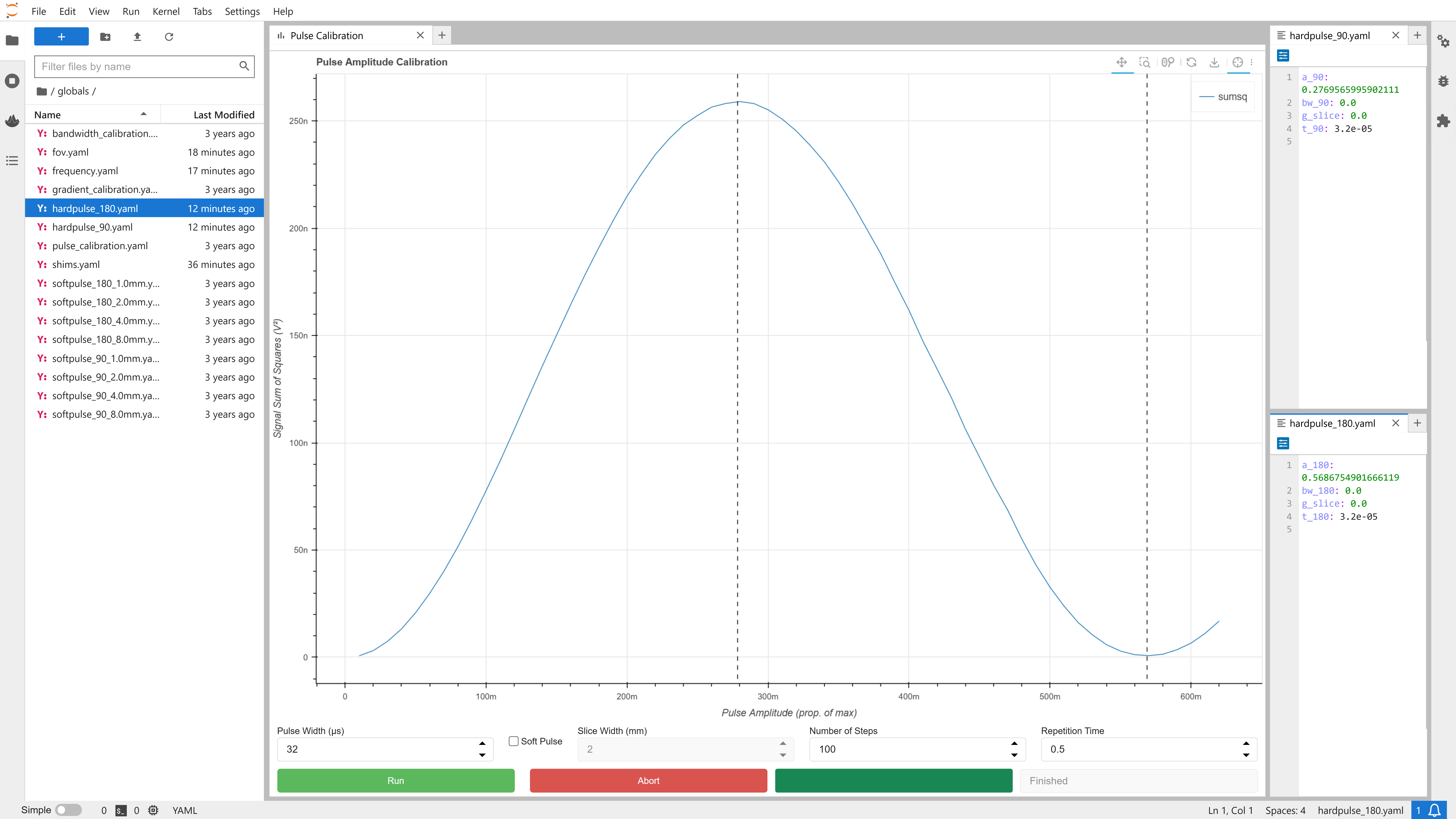
Pulse Calibration Dashboard
Autoshim
The final setup step is to determine the electrical shim settings, which is done using the Autoshim dashboard.
At the bottom left of the dashboard there is a dropdown menu with three options:
Coarse - This option starts the shimming process from scratch and should be used to shim the system each time it is powered on.
Quick - A Quick shim can be run periodically to re-optimise the homogeneity if it has drifted (due to small changing thermal gradients in the magnet).
Fine - Slower and more precise shim.
Select the coarse option and click Run.
The shim values are automatically saved to the following shims file (with values in the range [-1,1]):
globals/shims.yaml
Now that the system is setup and calibrated, it is time to begin your experiments!
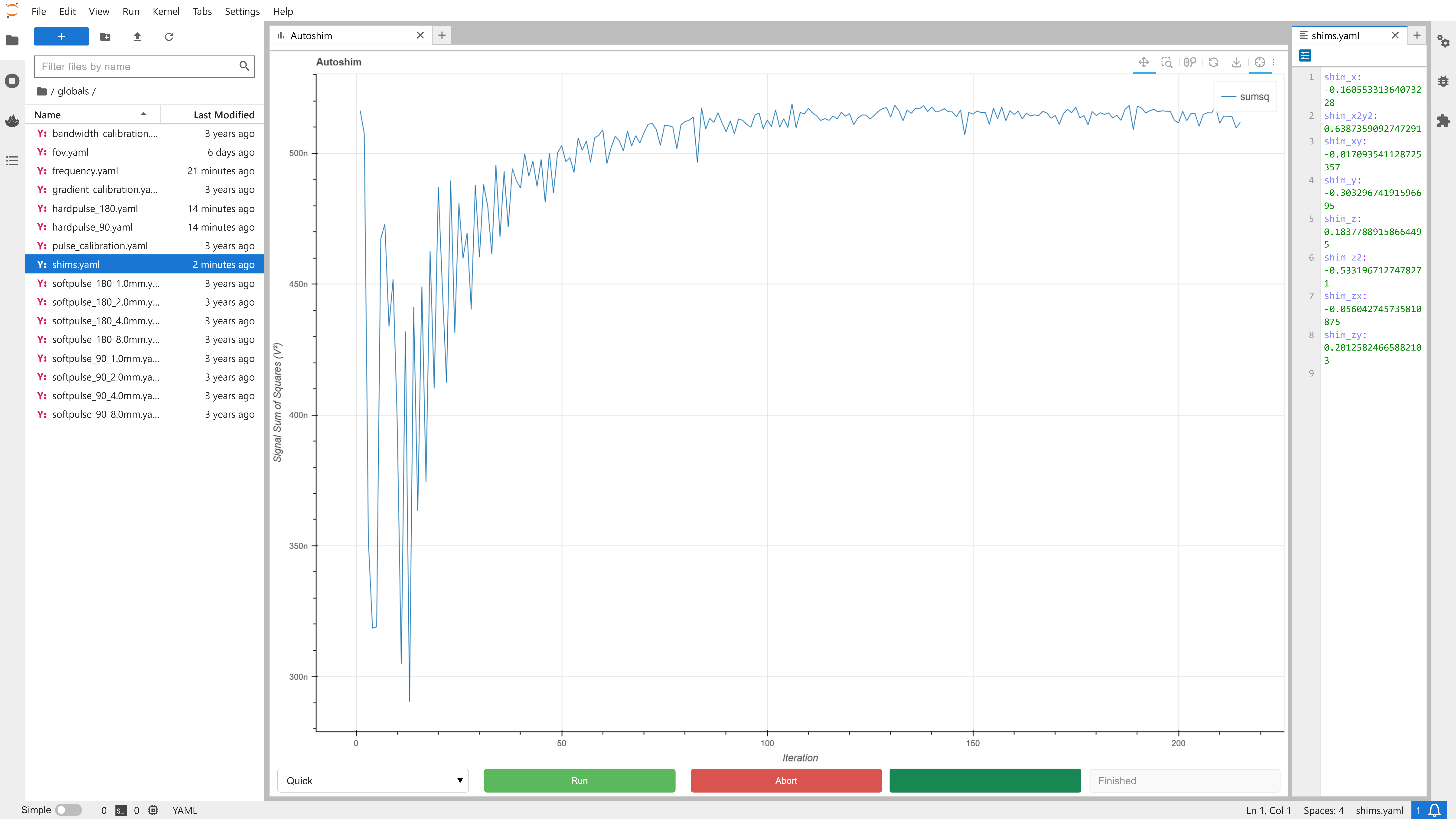
Autoshim Dashboard
Experiment Apps
The experiment apps allow you to run a series of NMR and MRI experiments with the click of a few buttons and immediately visualise results.
FID
This experiment runs a Free Induction Decay pulse sequence with the following parameters:
Scans - can be used to improve the signal-to-noise ratio (SNR) by averaging multiple scans.
Rep Time - time waited between scans, may need to be increased for samples with a long T1 recovery time (e.g. pure water).
Samples - number of complex samples acquired.
Dwell Time - time between samples, longer dwell time will result in a narrower bandwidth in the Spectrum plot on the right.
Acq. Delay - time delay after the RF pulse to allow for probe/duplexer dead time, should not need to be modified.
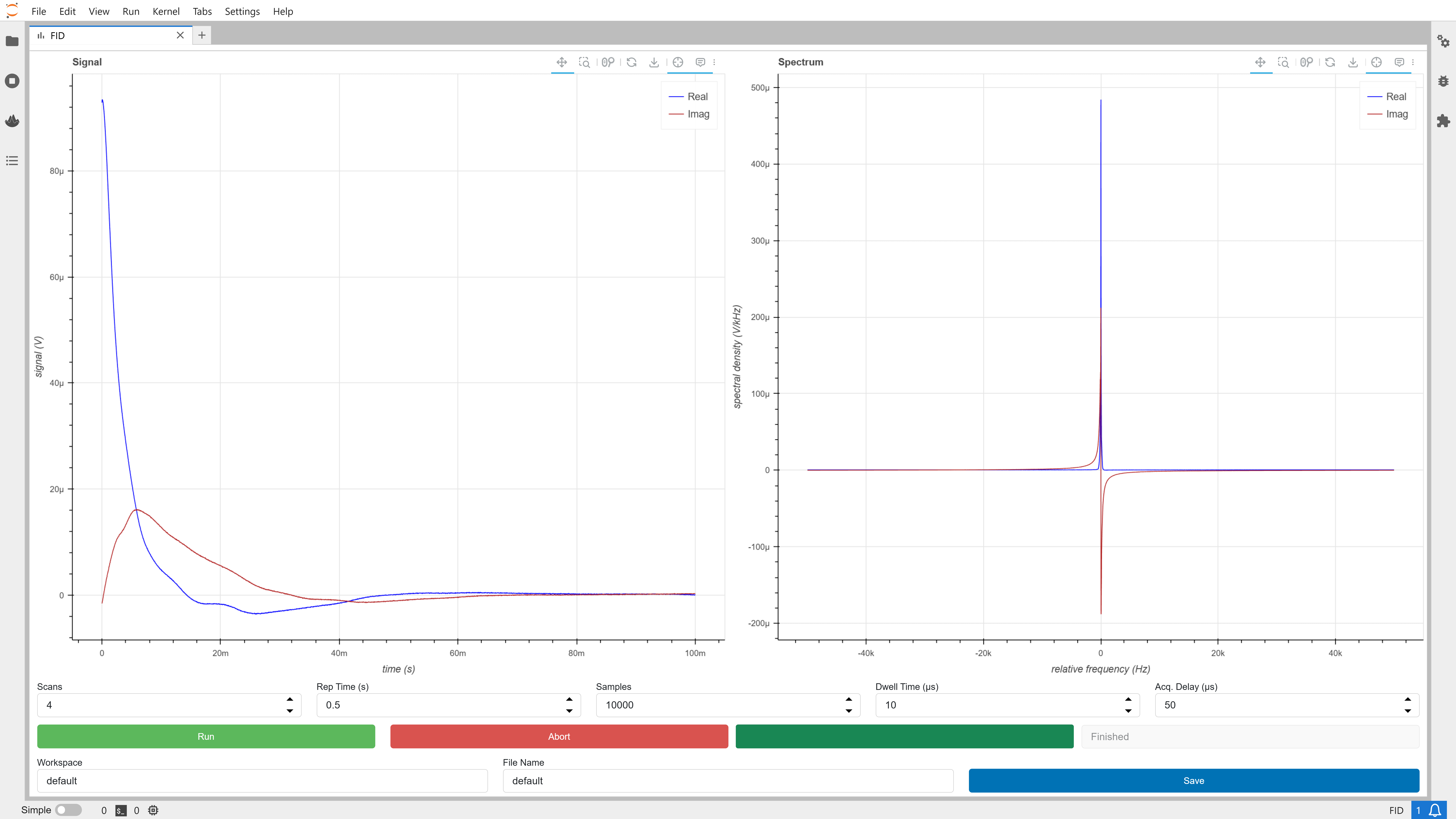
FID Dashboard
Note
Frequency, pulse power/width, and shim settings are read from the global system parameter files every time the experiment is run, and cannot be set manually in the dashboard.
CPMG
This experiment runs a Carr-Purcell-Meiboom-Gill pulse sequence, repeated “Scans” times with 2 or 4 step phase cycling with the following parameters:
Scans - can be used to improve the signal-to-noise ratio (SNR) by averaging multiple scans. Use 2 or a multiple of 4 scans for best results.
Rep Time - time waited between scans, may need to be increased for samples with a long T1 recovery time (e.g. pure water).
Samples - number of complex samples acquired per echo.
Dwell Time - time between samples.
Echo Time - time between 180 degree RF pulses, determines the time between data point on the Integrated Echos plot.
Echo Count - number of echos, determines number of points on the Integrated Echos plot.
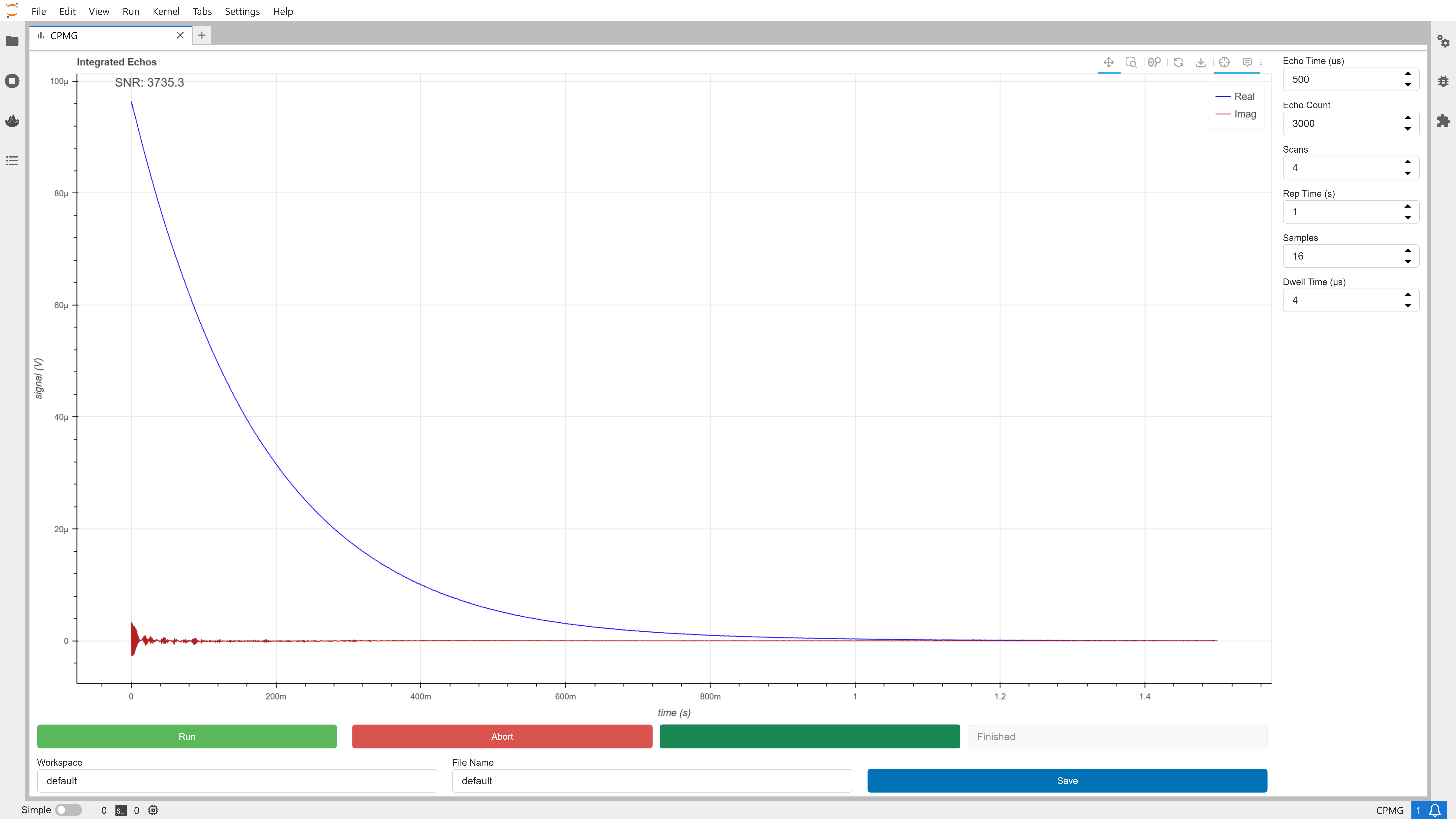
CPMG Dashboard
Note
Frequency and pulse power/width are read from the global system parameter files every time the experiment is run, and cannot be set manually in the dashboard.
1D SE
This experiment runs a Spin Echo pulse sequence with a frequency encoding gradient for 1D projection imaging, and optionally using soft 90 pulse with slice gradient for slice selection (can be applied along the same direction as the frequency encode gradient to measure the slice profile).
Parameters:
Scans - can be used to improve the signal-to-noise ratio (SNR) by averaging multiple scans.
Rep Time - time waited between scans, may need to be increased for samples with a long T1 recovery time (e.g. pure water).
Freq Enc Res - desired spatial resolution of the image along the frequency encode axis.
Freq Enc Axis - selects which gradient to use for frequency encoding, or no gradient if N.
Slice Width - desired spatial width of the slice.
Slice Offset - desired spatial offset of slice along the slice axis.
Slice Axis - selects which gradient to use for slicing, or no gradient if N. The experiment will use a hard 90 pulse when this option is set to N.
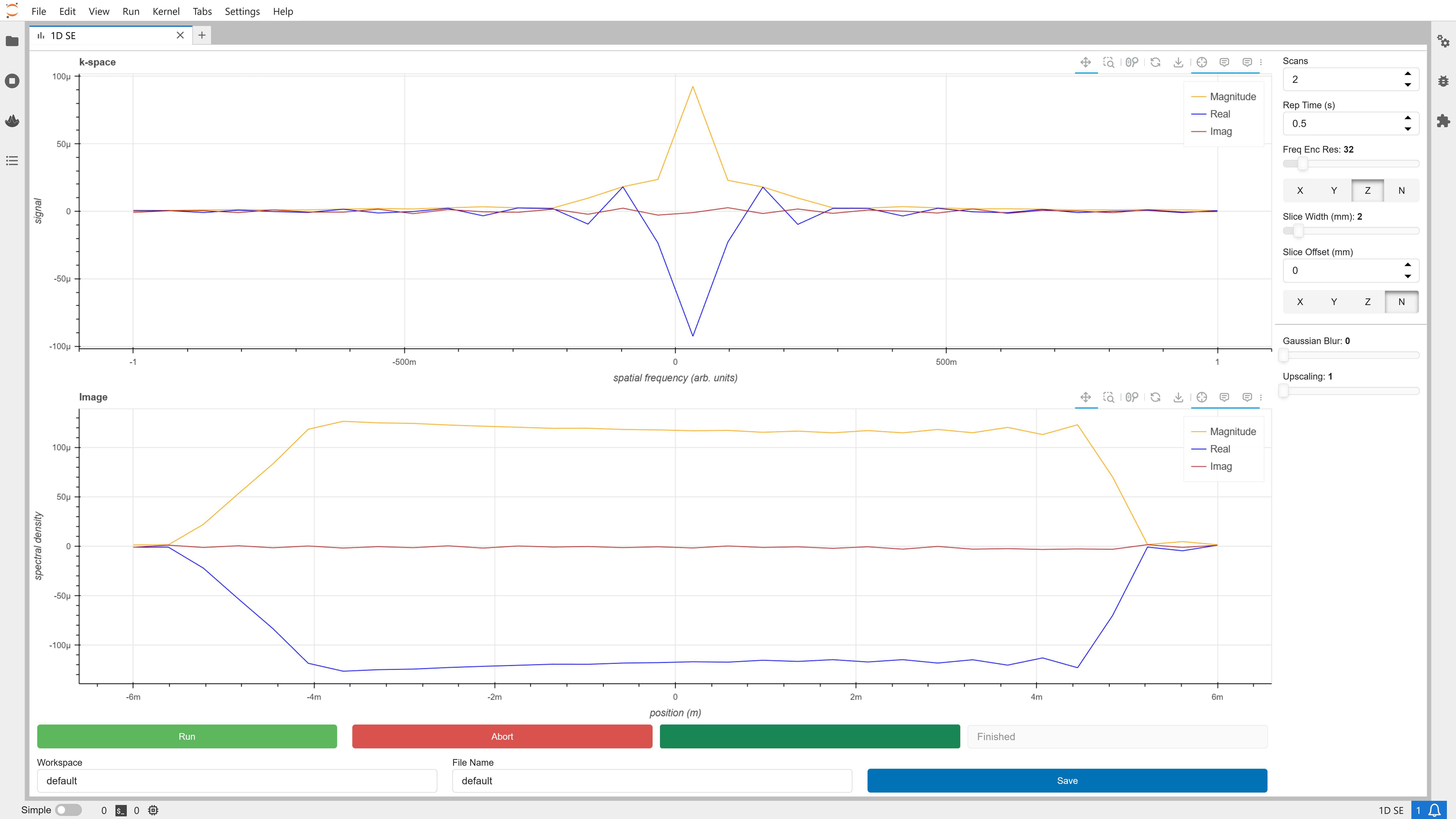
1D SE Dashboard
The following post processing parameters are for smoothing and scaling the data:
Gaussian Blur - windows the data prior to Fourier reconstruction to filter out high frequency artefacts and increase SNR at the expense of resolution. Use 0 for no blurring.
Upscaling - zero fills the data prior to Fourier reconstruction to reduce pixellation and give a smoother image. Use 1 for no upscaling.
Note
Frequency, pulse power/width, and shim settings are read from the global system parameter files every time the experiment is run, and cannot be set manually in the dashboard.
2D RARE
This experiment runs a RARE pulse sequence with optional slicing, frequency encode, and phase encode for either 2D projection or 2D slice imaging parameters:
Scans - can be used to improve the signal-to-noise ratio (SNR) by averaging multiple scans.
Rep Time - time waited between scans, may need to be increased for samples with a long T1 recovery time (e.g. pure water).
Freq Enc Res - desired spatial resolution of the image along the frequency encode axis.
Freq Enc Axis - selects which gradient to use for frequency encoding, or no gradient if N.
Phase Enc Res - desired spatial resolution of the image along the phase encode axis.
Phase Enc Axis - selects which gradient to use for phase encoding, or no gradient if N.
Slice Width - desired spatial width of the slice.
Slice Offset -
Slice Axis - selects which gradient to use for slicing, or no gradient if N. The experiment will use a hard 90 pulse when this option is set to N.
For more in details about these parameters, head over to our blog post: Selecting Imaging Parameters for RARE Pulse Sequences.
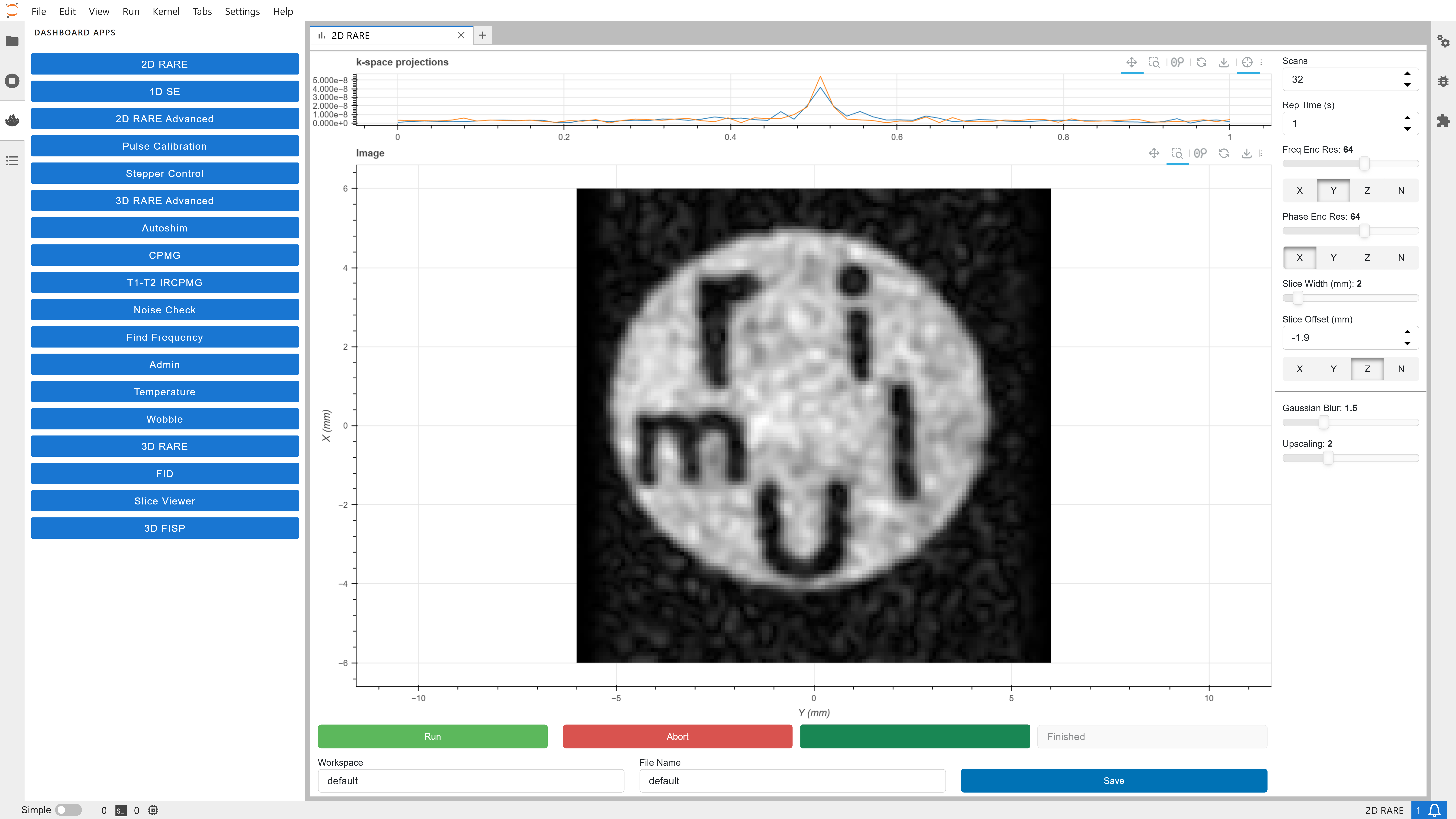
2D RARE Dashboard
The following post processing parameters are for smoothing and scaling the data:
Gaussian Blur - windows the data prior to Fourier reconstruction to filter out high frequency artefacts and increase SNR at the expense of resolution. Use 0 for no blurring.
Upscaling - zero fills the data prior to Fourier reconstruction to reduce pixellation and give a smoother image. Use 1 for no upscaling.
Note
Frequency, pulse power/width, and shim settings are read from the global system parameter files every time the experiment is run, and cannot be set manually in the dashboard.
2D RARE Advanced
The 2D RARE advanced dashboard is an expansion of the standard 2D RARE dashboard. The additional controllable parameters make it better suited for contrast imaging experiments.
As well as the standard 2D RARE parameters, 2D RARE Advanced includes the following parameters:
Echo Train Length (ETL) - number of echoes produced per scan.
Effective Echo Time (TE_eff) - time from 90 degree pulse to the echo that is acquired during the lowest order phase encode step, used in combination with Rep. Time to create T1,T2, and Proton weighted images.
Dummy Echo Enable (located under Rep. Time) - check to add a dummy (not acquired) echo module to the pulse sequence. If using a short Rep. Time, use a dummy echo to esure the longitudinal magnetization reaches a steady state before the first echo is acquired.
Inversion Recovery Enable - check to add an inversion recovery module to the pulse sequence.
Inv. Time - time from the inversion pulse to acquisition of the signal, any parts of the sample that have longitudinal magnetization close to zero at the end of the Inv. Time will be suppressed in the image.
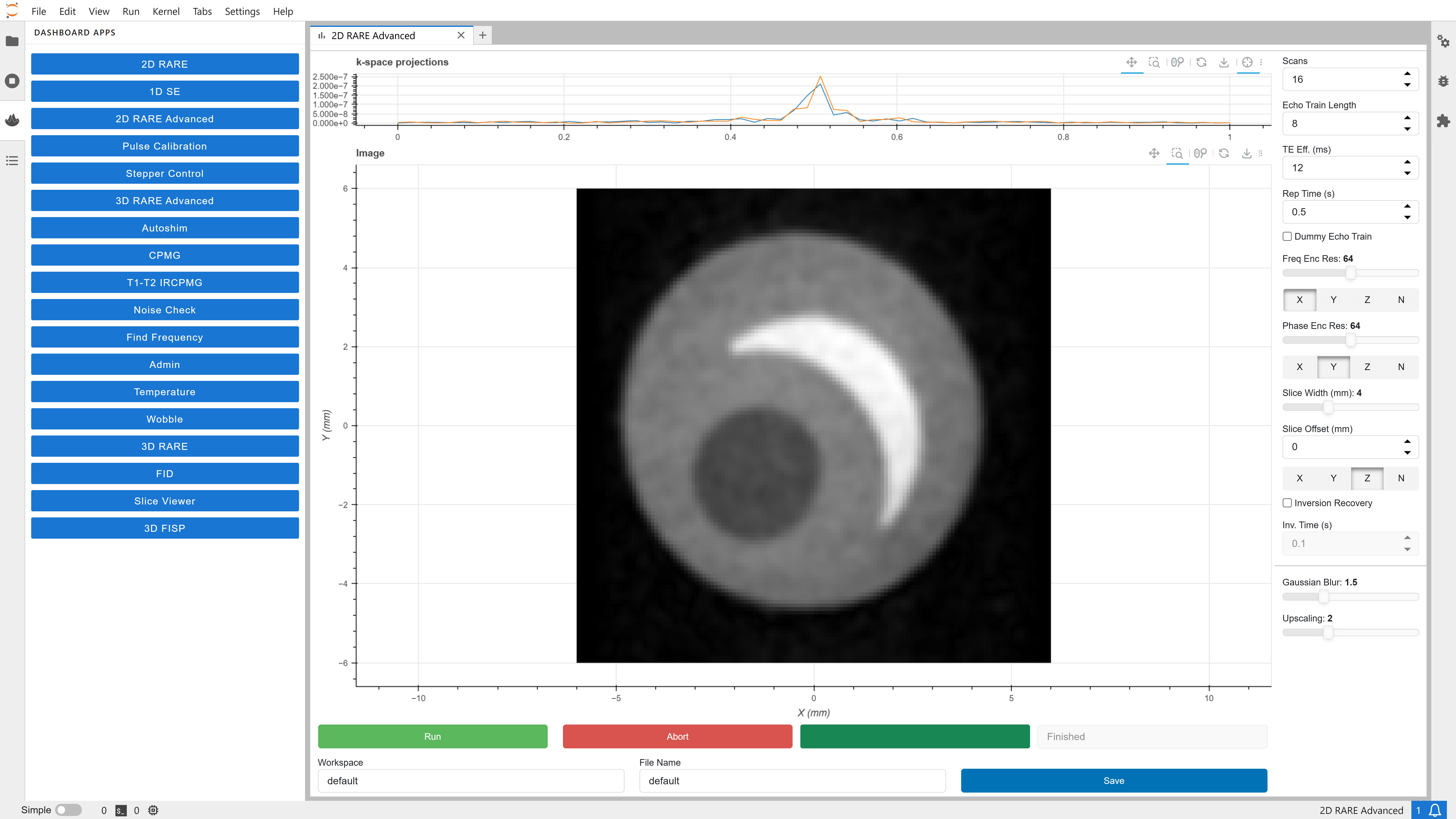
2D RARE Advanced Dashboard
3D RARE
This experiment runs a RARE pulse sequence with frequency encode along one axis and phase encode along two axes. The number of echos in the CPMG sequence is set by Phase Enc 2 Res and the whole CPMG sequence is repeated Phase Enc 1 Res times, with appropriate phase gradient pulses.
Parameters:
Scans - can be used to improve the signal-to-noise ratio (SNR) by averaging multiple scans.
Rep Time - time waited between scans, may need to be increased for samples with a long T1 recovery time (e.g. pure water).
Freq Enc Res - desired spatial resolution of the image along the frequency encode axis.
Freq Enc Axis - selects which gradient to use for frequency encoding, or no gradient if N.
Phase Enc 1 Res - selects which gradient to use for the first phase encoding, or no gradient if N.
Phase Enc 1 Axis - selects which gradient to use for phase encoding, or no gradient if N.
Phase Enc 2 Res - desired spatial resolution of the image along the second phase encode axis.
Phase Enc 2 Axis - selects which gradient to use for the second phase encoding, or no gradient if N.
For more in details about these parameters, head over to our blog post: Selecting Imaging Parameters for RARE Pulse Sequences.

3D RARE Dashboard
The following post processing parameters are for smoothing, scaling, and viewing the data:
Gaussian Blur - windows the data prior to Fourier reconstruction to filter out high frequency artefacts and increase SNR at the expense of resolution. Use 0 for no blurring.
Upscaling - zero fills the data prior to Fourier reconstruction to reduce pixellation and give a smoother image. Use 1 for no upscaling.
View Slice index - set the slice axis with the F/P1/P2 radio buttons (physical axis will depend on above settings) and drag the View Slice Index slider to move the slice plane through the 3D data.
Note
Frequency, pulse power/width, and shim settings are read from the global system parameter files every time the experiment is run, and cannot be set manually in the dashboard.
3D RARE Advanced
The 3D RARE advanced dashboard is an expansion of the standard 3D RARE dashboard. The additional controllable parameters make it better suited for contrast imaging experiments.
As well as the standard 3D RARE parameters, 3D RARE Advanced includes the following parameters:
Echo Train Length (ETL) - number of echoes produced per scan.
Effective Echo Time (TE_eff) - time from 90 degree pulse to the echo that is acquired during the lowest order phase encode step, used in combination with Rep. Time to create T1,T2, and Proton weighted images.
Dummy Echo Enable (located under Rep. Time) - check to add a dummy (not acquired) echo module to the pulse sequence. If using a short Rep. Time, use a dummy echo to esure the longitudinal magnetization reaches a steady state before the first echo is acquired.
Inversion Recovery Enable - check to add an inversion recovery module to the pulse sequence.
Inv. Time - time from the inversion pulse to acquisition of the signal, any parts of the sample that have longitudinal magnetization close to zero at the end of the Inv. Time will be suppressed in the image.
3D RARE Advanced Dashboard
3D FISP
This experiment runs a FISP (also called GRASS) pulse sequence with frequency encode along one axis and phase encode along two axes.
Parameters:
Scans - can be used to improve the signal-to-noise ratio (SNR) by averaging multiple scans.
TR - time between RF pulses; affects T1 contrast and pulse sequence duration.
Flip Angle - sets the flip angle of the RF pulse used.
Freq Enc Res - desired spatial resolution of the image along the frequency encode axis.
Freq Enc Axis - selects which gradient to use for frequency encoding, or no gradient if N.
Phase Enc 1 Res - desired spatial resolution of the image along the first phase encode axis.
Phase Enc 1 Axis - selects which gradient to use for the first phase encoding, or no gradient if N.
Phase Enc 2 Res - desired spatial resolution of the image along the second phase encode axis.
Phase Enc 2 Axis - selects which gradient to use for the second phase encoding, or no gradient if N.
3D FISP Dashboard
The following post processing parameters are for smoothing, scaling, and viewing the data:
Gaussian Blur - windows the data prior to Fourier reconstruction to filter out high frequency artefacts and increase SNR at the expense of resolution. Use 0 for no blurring.
Upscaling - zero fills the data prior to Fourier reconstruction to reduce pixellation and give a smoother image. Use 1 for no upscaling.
View Slice index - set the slice axis with the F/P1/P2 radio buttons (physical axis will depend on above settings) and drag the View Slice Index slider to move the slice plane through the 3D data.
Note
Frequency, pulse power/width, and shim settings are read from the global system parameter files every time the experiment is run, and cannot be set manually in the dashboard.